We’re excited to share the story behind the development of DL Backtrace - our Mode-agnostic explainability technique, purpose-built for deep learning models. DLBacktrace (Arxiv & Github), developed by AryaXAI, introduces a novel approach to interpreting model behavior across any modality or scale. By precisely tracing the relevance of model decisions back to their inputs, it reveals detailed insights into the internal workings of models—from individual parameters and layers, down to tokens in large language models (LLMs).

This deterministic and architecture-independent framework brings a new level of transparency, reliability, and robustness—making it especially valuable in mission-critical domains like finance, healthcare, and compliance-driven AI deployments.

In this session, we’re joined by Pratinav Seth, Research Scientist at AryaXAI, who will walk us through:

• The motivation behind DL Backtrace
• How the method works under the hood
• Comparisons with traditional interpretability techniques
• Real-world benchmarks across tabular, vision, and NLP tasks
• And how you can start using it today

Let’s dive in!

Papers and Resources Discussed:

• DL Backtrace Paper: https://arxiv.org/abs/2411.12643v1 
• Github: https://github.com/AryaXAI/DLBacktrace?tab=readme-ov-file 
• XAI Evals: https://arxiv.org/html/2502.03014v1 

Transcript:

Sugun Sahdev:
Welcome everyone, and thank you for joining AryaXAI’s webinar Inside the Black Box: Interpreting LLMs with DL Backtrace. I’m Sugun, your host today. We’re excited to share our latest work in explainable AI.

Today’s agenda includes a quick overview of AryaXAI, followed by a deep dive into DL Backtrace, a notebook walkthrough, and a live Q&A.

Sugun Sahdev:
To get us started, I’d like to invite Pratinav, a research scientist at AryaXAI and the author of the DL Backtrace library. Pratinav, over to you.

Pratinav Seth:
Thanks, Sugun. Hello everyone! I'm Pratinav. So, DL Backtrace is a method through which you can do model-agnostic explainability. In today's session, we'll focus particularly on LLMs and the fundamentals of DL backtrace. 

I currently work as a research scientist at AryaXAI alignment labs. I'm currently working around interpretability alignment and other real-world tasks, which we are dealing with at AryaXAI. 

Let me begin with the AI Alignment Lab. We're based in Mumbai and Paris and are dedicated to building research-grade tools to address AI alignment and interpretability. The reason being how they are very important in today's world and with all these regulations coming up in different parts of the world, it leads to further more questions, how you can actually interpret different AI models which are coming up every week and how you can build on these new techniques so that you can ensure the models which you're using are safe to use as well as well aligned.

Our current approach works around building new techniques to solve these problems, how you can work on open source tools so that the industry has tools to solve certain problems, as well as have enough tools on AI safety. Alongside that, we also work on open source tools. We have two tools, which are DL Backtrace and Xai Evals. Alongside that, we also collaborate with the academic and research labs.

We're also hiring for a couple of positions around research, as well as software development and more. If in case you're interested in our vision, please feel free to contact us or me.

Pratinav Seth:
So coming with this, like what's the main problem in AI? Every day you have different teams or, you have different organizations creating domain specific models. However, I would say the huge impact it is causing number of people who are actually using these models. 

The problem is, especially in mission critical tasks like let's say in finance, the use of AI is very sensitive because it can lead to quite high monetary impact as well as in other domains as well there is a very high impact on using AI, especially let's say medical, let's say manufacturing can lead to large scale impacts. It is very critical and it can lead to other problems as well if you're using it in everyday life, which is mostly around, let's say manipulation and other stuff. And the reason why all this is important and why we are working around this area is that there's not much which has been done around AI safety and alignment, making it a very important problem and something which needs fundamental research to solve.

For mission-critical ‘AI’, buidling models is easy; But model acceptance is hard!

You can build a new model every day with fresh data, but the real challenge lies in ensuring that the model is transparent and compliant with AI regulations across different jurisdictions. As global regulatory frameworks around AI continue to emerge, it becomes critical to address not only how the model performs but also how it communicates failure. If a model fails, how do you ensure that the end users are appropriately informed?

A model must earn the trust of all stakeholders—product and operations leaders, risk and audit teams, financial officers, and, importantly, the customers. For that trust to be established, the AI must behave fairly, transparently, and consistently. It cannot be random or unpredictable; it must be deterministic, meaning that given similar input data, the output should remain consistent.

The model must also meet all applicable regulatory requirements, particularly those set by government bodies. It should be free from bias and offer clear, explainable decisions. Ultimately, customers and stakeholders need confidence that the model's outcomes are not only accurate but also justifiable and fair.

So why is there a problem of AI explanation, or a problem of AI alignment, or interpretability?

The reason being, there are methods to explain different models, but they are not always correct—or I would say, often provide wrong explanations—which creates distrust among users. Another problem is that these methods are not acceptable in many cases because a lot of the models are black boxes, which makes it very hard for any method to properly explain them.

And secondly, it’s very hard to debug the problems with these explanation methods. Now, in current times, there’s a lot more maturity when it comes to AI regulation and governance, especially in Europe. We already have a traditional, or you could say milestone-based, AI regulation act that’s come up and will be in effect starting next year. In the US, a lot of regulations are also coming up. Similarly, in countries like Canada and China, there’s a different kind of regulatory framework, and .in India, there’s something that might be introduced in the next few months.

So, I would say there’s a growing realization among different governments that with the increasing use of AI in everyday life, there needs to be regulations and governance frameworks that these AI models must align with.

This brings us to a fundamental problem in AI today—the black box nature of most models.

The "Black Box" Problem in AI

We know that a model might perform well, but understanding how it arrives at a decision is still a big challenge. The reason is that most of these models are built on neural networks which often have millions of parameters and perform a vast number of operations internally. This makes them extremely difficult to interpret—they become black boxes.

Now, there are several explanation methods out there—some are model-agnostic like LIME and SHAP, while others are gradient-based, like GradCAM and Integrated Gradients. But again, none of these work across all models or tasks. They’re usually very specific to a particular task or model architecture. 

Current XAI Limitations:

• Model-Agnostic (LIME, SHAP): Often costly, sensitive to data changes, struggle with complex data.
• Gradient-Based (Grad-CAM, Integrated Gradients): Architectural limits, depend on baselines, complex to interpret.
• Lack of Unified Metrics: Difficult to compare methods; can lead to conflicting explanations.

And the second important challenge is: how do we evaluate these explanation methods? That’s still not very clear. There are some metrics available, yes—but there’s no unified standard for evaluation across different use cases. So why is this becoming a major issue now? Why wasn’t it as much of a concern five years ago?

The reason is that with the exponential increase in the complexity of models, our ability to understand them hasn’t kept pace. So, even though these models perform incredibly well, we are increasingly unable to understand how they actually work.  And that brings us to the question—what are the explanation methods available today?

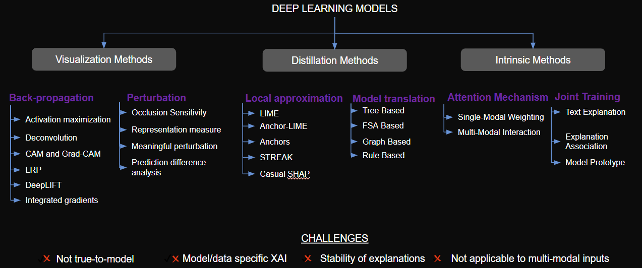
Current explainability methods

Pratinav Seth [09:25]:

So, as you can see in the chart, there are various methods that have been developed to explain deep learning models. First, we have visualization methods, including perturbation-based techniques, which are quite popular. These involve modifying parts of the input to observe how the model's predictions change, essentially trying to "trick" the model to understand how it's making decisions.

Then there are local approximation methods, like LIME and SHAP, which are widely used. These rely on surrogate modeling—creating simpler, interpretable models around a prediction to estimate feature importance.

We also have tree-based model translation methods, shown under distillation in the figure. These reflect traditional ML thinking and offer clear decision paths. And that’s why, especially in high-stakes domains like finance and healthcare, people still tend to prefer tree-based models—they’re easier to explain. The challenge is that this level of transparency doesn’t carry over to deep learning models.

Then we have attention mechanisms, which people often point to as explanations in modern models. But attention weights weren’t designed for interpretability—they don’t directly explain the decision process.

Lastly, there’s joint training, a relatively newer area. These methods aim to train models that learn how to explain themselves while learning the task. It's an exciting direction, but still early.

Now, the issue with all of these approaches is—they come with significant limitations. Many are not model-agnostic, and most don’t generalize across domains. They also often don’t work with multimodal inputs, which are increasingly common. As we move toward more multimodal systems, this becomes a major gap. Another issue is the stability of the explanations. In many cases, the same model can yield different explanations for similar inputs. And, crucially, many of these methods are not true to the model—they interpret a proxy, not the actual behavior. So, keeping all this in mind, let’s quickly walk through some of the commonly used methods.

LIME, for example, is a local surrogate modeling technique. It’s probably one of the most widely used explanation methods today. SHAP builds on Shapley values and is another common approach for explaining predictions, especially in tabular data. These methods do offer some insight into what features matter, but they often fail on a case-by-case basis.They don’t reflect what the model is actually doing for a specific instance. Instead, they generalize based on feature importance, which can be misleading. Plus, they can be easily fooled through adversarial perturbation attacks—this is a known vulnerability.

Next, we have GradCAM, which is very common in vision models. But it mostly works for classification tasks. You can try to adapt it to segmentation, but beyond that, its use is limited. Integrated Gradients is another popular method. It's been used with models like LLaMA but it has its issues. It's heavily dependent on the baseline you choose. And for large models with deep gradient paths, the computational overhead becomes significant. So yes, it works with many architectures, but it's not a stable or scalable explanation method.

SmoothGrad is in a similar space—also mainly used in vision, but extendable to other domains. Then there’s LRP—Layer-wise Relevance Propagation. This method redistributes the prediction score layer by layer back to the input features. It supports various architectures and tasks, but it’s very computationally expensive, and tightly coupled to neural network internals, making it hard to scale.

Current XAI Limitations:

• Model-Agnostic (LIME, SHAP): Often costly, sensitive to data changes, struggle with complex data.
• Gradient-Based (Grad-CAM, Integrated Gradients): Architectural limits, depend on baselines, complex to interpret.
• Lack of Unified Metrics: Difficult to compare methods; can lead to conflicting explanations.

 So again, we come back to the same fundamental issue:

AI models today are still largely black boxes—and current explanation methods either don’t scale, aren’t faithful to the model, or don’t apply across tasks and modalities.

This is exactly the gap we set out to address with DL Backtrace.

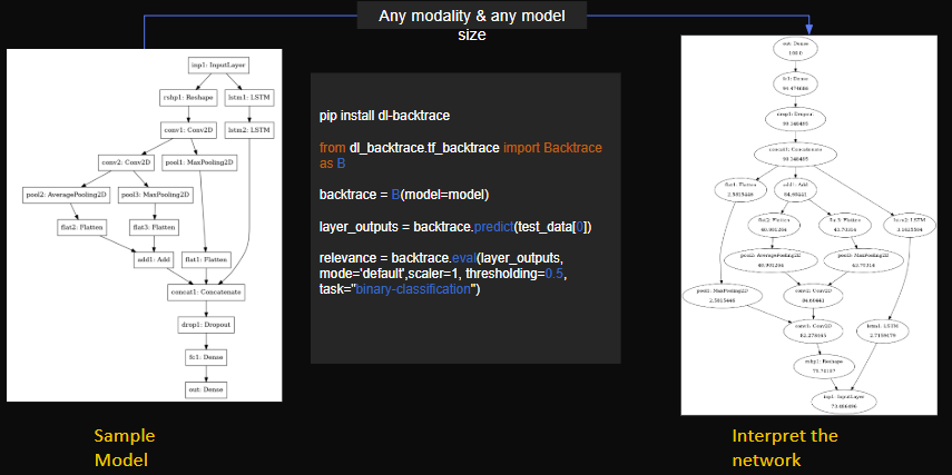
Introducing DLBacktrace – a Model Agnostic Explainability technique for Deep Learning Models

So, there’s a clear black box problem in AI today—and the challenge is, how do we solve this with a model-agnostic explainability approach?

To address that, we developed DL Backtrace—a model-agnostic explanation technique.By model-agnostic, I mean that you can apply it to any model architecture, and still be able to understand how the model works and how it arrives at a particular decision.

Now, you might ask—why create something new when we already have methods like LRP?

The reason is, we wanted something that’s more extensible—something that doesn’t rely on a set of predefined rules for different layers. In LRP, you need to specify certain rules for each type of layer, which adds complexity and limits scalability.

DL Backtrace, in contrast, uses a single, unified rule that can be applied across all layers. It’s simple, consistent, and stable.Our main goal was to develop an explanation algorithm that is independent of the model architecture and task. It should rely only on the learned model weights and the input data—nothing else. And it should quantify the contribution of each unit in the network, so you can clearly see how much each component is influencing the output.

Once you have that, you can meaningfully interpret the model by identifying which components are truly important.

DLBacktrace – How does it work?

So, how does DL Backtrace actually work—and why is it called “Backtrace” in the first place? Let’s start with the basics. In a typical neural network, you have a model architecture—represented here by the blue blocks—and during inference, you perform a forward pass to get the output.

In training, you then apply backpropagation, using gradients to update the model weights.

Now, in a similar fashion, what we do in DL Backtrace is:We calculate a relevance score starting from the output, and instead of propagating gradients, we backpropagate relevance—or, in our terminology, we backtrace it—through the network, using a custom rule that we’ve defined.

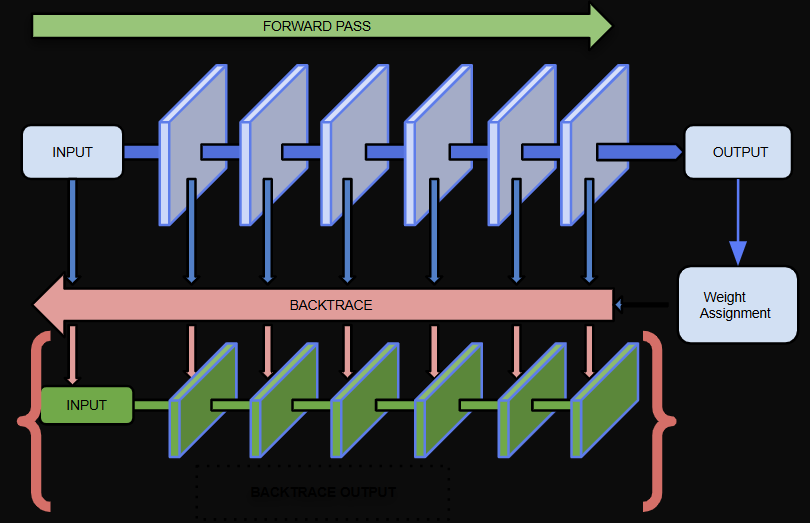
This rule allows us to assign relevance values to each operation or layer in the model, tracing back through the network to identify where the important contributions originated.

A helpful analogy here is Kirchhoff’s Law from electrical circuits—where current is conserved at each node. Similarly, DL Backtrace conserves relevance across operations, ensuring the attribution is consistent throughout the model.The result is an explanation map that aligns with your input space—highlighting which parts of the input, and which components of the network, contributed most to the model’s decision.

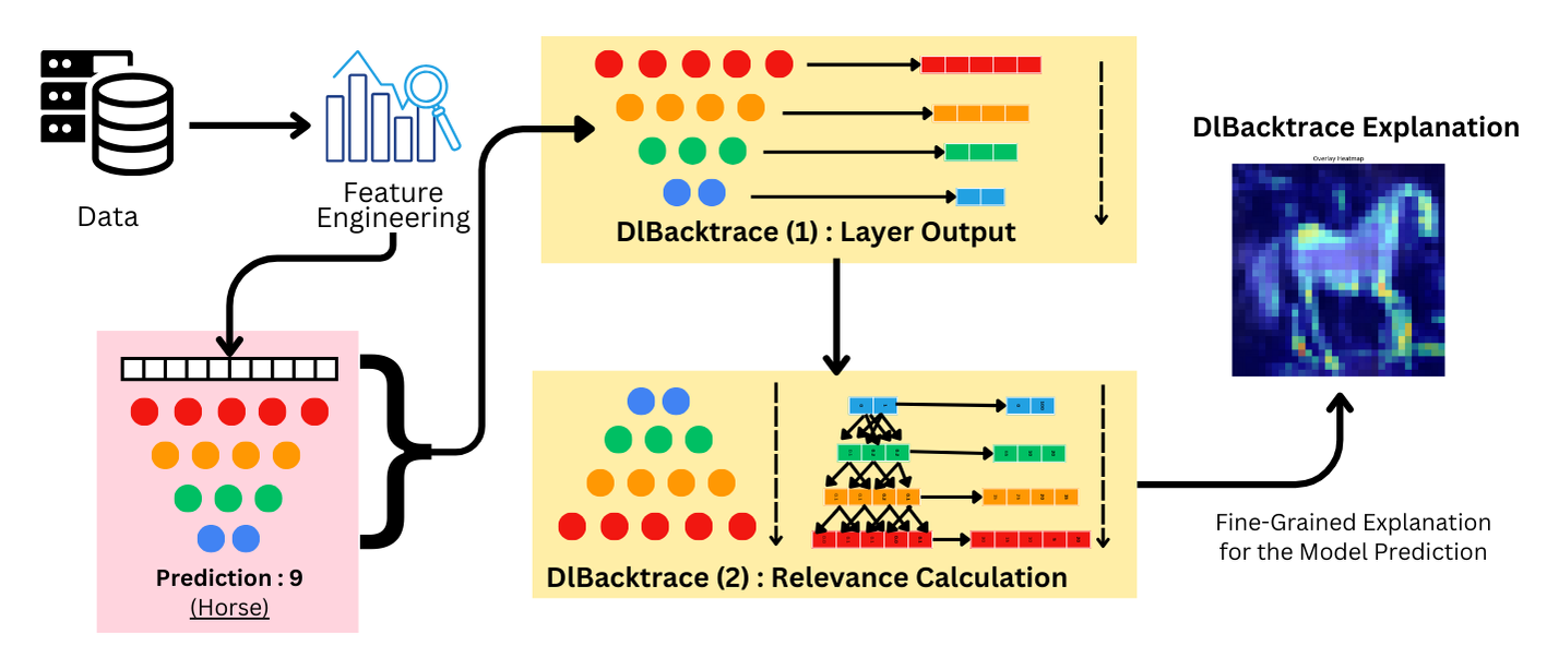
To give you a clearer picture:
You start with your data, apply any feature engineering, pass it through the model, and collect the outputs. Then, rather than looking only at the final result, DL Backtrace traces relevance values back through each layer using the model’s actual weights and structure.

This produces a detailed attribution—showing not just what the model predicted, but why it arrived at that prediction.

Along the way, we also quantify the importance of each layer in the network. That gives you additional insight, which can be used for downstream tasks like pruning, optimization, or auditing.

Algorithm Introduction:

Every neural network consists of multiple layers. Each layer has a variation of the following basic operation:

y = Φ(Wx + b)

where, Φ = activation function, W = weight matrix of the layer, b= bias, x  = input, y  = output

This can be further organized as: 

y = Φ(Xp + Xn + b)

where,

Xp = ∑Wixi ∀ Wixi > 0

Xn = ∑Wixi ∀ Wixi < 0

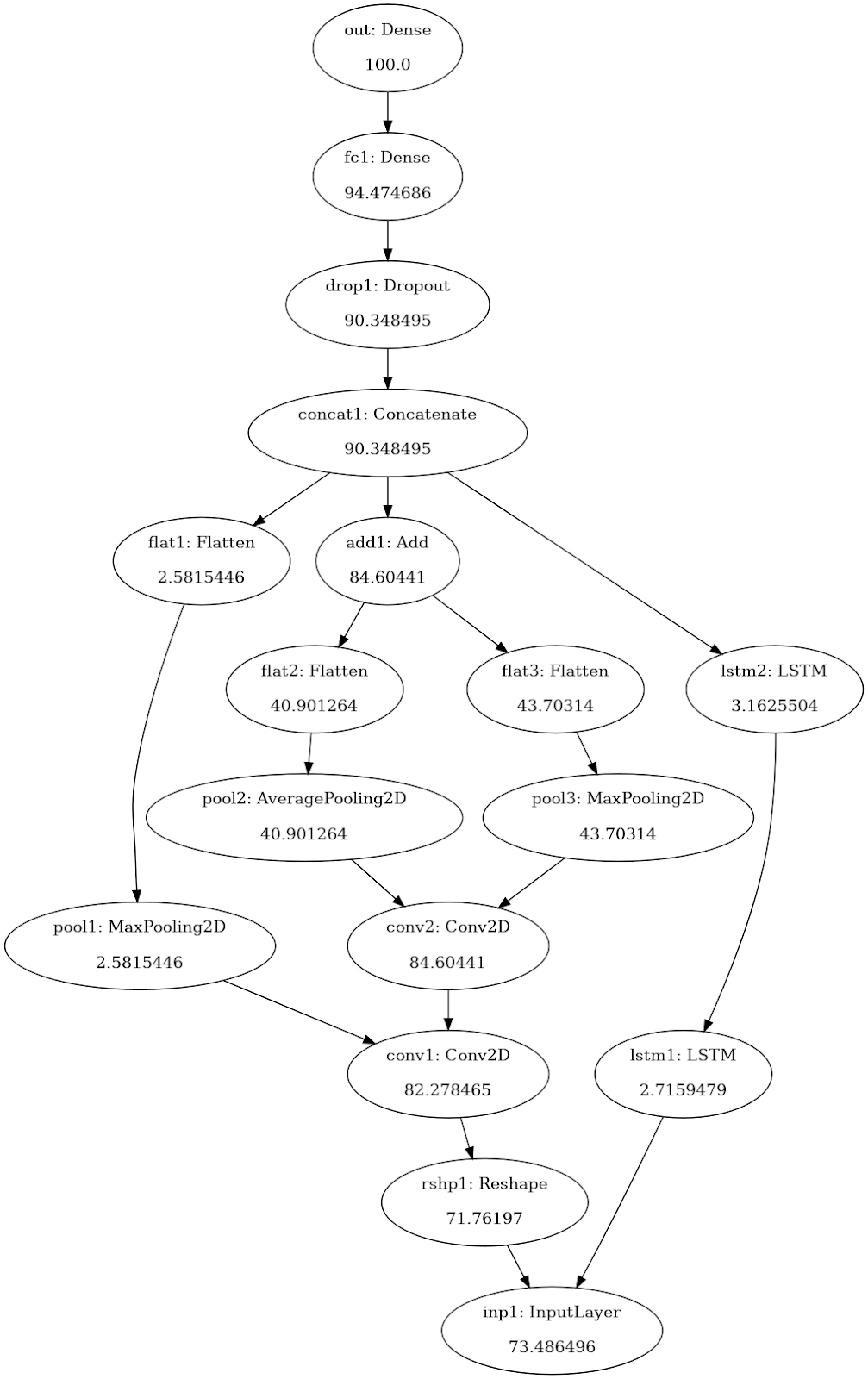
DLBacktrace Calculation for a Sample Network:

1. From the model weights and architecture, construct a graph with output nodes at the root and input nodes in the leaves.
2. The propagation starts at the root and proceeds in a breadth-first manner to avoid re-processing of any node.
3. The propagation completes when all the leaves(input nodes) have been assigned relevance. 
4. Any loss of relevance during propagation is due to network bias.
5. The relevance of a single sample represents local importance. For global importance, the relevance of each feature can be aggregated after normalization on the sample level.

We use two modes:

1. Default Mode: There is a single relevance associated with each unit. This is propagated by proportionately distributing the relevance between positive and negative components. If the relevance associated with y is r_y and with x is r_x, then for jth unit in y:

T^j = X_p^j + |X_n^j| + |b^j|

R_p^j = (X_p^j/T^j)r_y^j , R_n^j = (X_n/T^j)r_y^j , R_b^j = (b^j/T^j)r_y^j 

R_p^j and  R_n^j are distributed among x in the following manner,

r_xi^j = (W_i^jx_i^j/X_p^j)R_p^j ∀   W_i^jx_i^j > 0

        0        ∀   W_i^jx_i^j > 0 if Φ is saturated on negative end

        (-W_i^jx_i^j/X_n^j)R_n^j  ∀   W_i^jx_i^j < 0

        0       ∀  W_i^jx_i^j < 0 if Φ is saturated on positive end

        0      ∀  W_i^jx_i^j = 0

       ‍r_xi = ∑^jr_xi^j  .  Total relevance at layer x, r_x = ∑ⁱr_xi

The result is a layer-wise relevance value that reflects the overall importance of that layer in the model's decision-making process.

2. Contrastive Mode: In this there are dual relevance associated with each unit. This is propagated by proportionately distributing the relevance between positive and negative components. If the relevance associated with y are r_yp , r_yn and with x are r_xp , r_xn , then for jth unit in y:

T^j = X_p^j + X_n^j + b^j

if T^j > 0, then

if r_yp^j > r_yn^j: else:

R_p^j = r_yp^j R_p^j = r_yn^j

R_n^j = r_yn^jb R_n^j = r_yp^j

relevance_polarity = 1 relevance_polarity = -1

else

if r_yp^j > r_yn^j: else:

R_p^j = r_yn^j R_p^j = r_yp^j

R_n^j = r_yp^j R_n^j = r_yn^j

relevance_polarity = -1 relevance_polarity = 1

R_p^j and R_n^j are distributed among x in the following manner,

if relevance_polarity > 0, then else:

r_xp,i^j = (W_i^jx_i^j/X_p^j)R_p^j  ∀ W_i^jx_i^j > 0                         r_xp,i^j = (-W_i^jx_i^j/X_n^j)R_n^j ∀ W_i^jx_i^j < 0

r_xn,i^j = (-W_i^jx_i^j/X_n^j)R_n^j ∀ W_i^jx_i^j < 0 r_xn,i^j = (W_i^jx_i^j/X_p^j)R_p^j ∀ W_i^jx_i^j > 0

Thus,

r_xp,i = ∑^jr_xp,i^j

r_xn,i = ∑^jr_xn,i^j 

Total relevance at layer x: 

Positive relevance r_xp = ∑ⁱr_xp,i 

Negative relevance r_xn = ∑ⁱr_xn,i

In this mode, we still compute the total relevance, but we go a step further—we separate the positive and negative contributions. For example, if the negative contribution is greater than the positive one, we use a different computation strategy to reflect that. Likewise, if the positive contribution outweighs the negative, we handle it differently.

The goal here is to clearly distinguish what parts of the network are contributing positively toward the model’s decision and what parts are contributing negatively. This allows us to compute not just a single relevance score, but both the positive and negative relevance at each node.

Now, why introduce contrast mode at all? Why not just stick with the default?

The reason is that in certain scenarios—especially when you're analyzing edge cases or borderline decisions—it becomes critically important to understand both sides:

• What supported the model’s prediction
• And what opposed it

Contrast mode helps surface that level of nuance by showing the exact reasons that pushed the model toward or away from a particular outcome.

Attention Layers

In addition to everything we've discussed so far, one important enhancement we made was specifically for attention layers—which are central to all modern LLMs, including models like BERT and other attention-based architectures that are becoming increasingly common today.

This was a crucial step, given how essential attention mechanisms are in these models.So, in attention layers—particularly multi-head attention—you have components like query, key, and value, which together define the soft attention mechanism.

What we do in DL Backtrace is compute relevance by analyzing both the query-value and query-key interactions.This approach is inspired by the Attention Library paper, and we extend that concept by calculating the relevance scores for query, key, and value independently.

• The attention function employs the equations:

Attention(Q, K, V) = softmax((QK^T)/√d_k)V

• For Multi-Head Attention, it becomes _i^Q

MultiHead(Q, K, V) = Concat(head₁, head₂, …, head_h) W^o

• where each head is computed as:

head_i = Attention(QW_i^Q_, KW_i^K, VW_i^V)

• Such that:
  
  • Q, K, V : Query, Key, and Value Matrices
  • W_i^Q_,  W_i^K, W_i^V :  Weight matrices for the i-th head
  • W^o : Weight matrix for combining all the heads after concatenation
  • Concat: Concatenation of the outputs from all attention heads

• Suppose, the input to the attention layer is x and output is y. The relevance associated with y is r_y.

To compute the relevance using Backtrace,

• First, we calculate the r_O of Concat(head₁, head₂,.., head_h) [as given in earlier].  r_O represents the relevance from the linear projection layer of the Attention module..
• To compute the relevance of QK^T  and V, we use the following formula [taken from AttnLRP]:

r_QK = (r_O * x_V) . x_QK & r_V = (x_QK * r_O) . x_V   

Here, x_QK and x_V are the outputs of QK^T  and V, respectively.

• Now, we have r_QK, we will compute the relevance of r_Q and r_K as:

r_Q = (r_QK * x_Q) . x_K & r_K = (x_K * r_QK) . x_Q

Here, x_Q and x_K are the outputs of Q and K, respectively.

• To compute the r_Attn, we will sum up the r_Q, r_K and r_V.

r_Attn = r_Q + r_K + r_V

The result is a summed relevance score for the entire attention layer, giving us a clear attribution of how each part of the attention mechanism contributed to the final decision.

That wraps up our explanation of how DL Backtrace handles attention layers. Now, let’s move on to the benchmarking.

Benchmarking Explainability Methods:

Pratinav Seth:

Once we had DL Backtrace in place, the next big question was—how do we know if it actually works? To validate the method, we benchmarked it across three different types of tasks: tabular, image, and text:

1. Tabular : 

• Problem Statement: Lending Club Dataset (Binary Classification) using 3 Layer MLP Neural Network.
• Metrics: MPRT & Complexity.

2. Image :

• Problem Statement: CIFAR-10 (Multi Class Classification) using Supervised Fine Tuned ResNet 34.
• Metrics: Pixel Flipping, Faithfulness Correlation & Max Sensitivity.

3. Text :

• Problem Statement: SST-2 Binary Classification using Pre-Trained BERT.
• Metrics: Token Perturbation for Explanation Quality (ToPEQ) (~ Pixel Flipping).

Let’s discuss the metrics we used for evaluation.

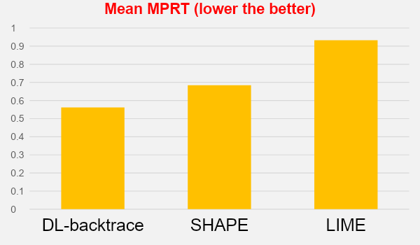
Starting with the tabular benchmarks, we used two key metrics: MPRT and complexity.

• Maximal Perturbation Robustness Test (MPRT) measures how much perturbation can be applied to an input before the explanation of the model's decision changes significantly. It helps assess the stability and robustness of the model's explanations, not just its predictions.
• Complexity metric measures how detailed a model's explanation is by calculating the distribution of feature contributions.

Moving on to the image modality, we used:

• Faithfulness Correlation: Measures how well an explanation aligns with a model’s behavior by computing the correlation between feature importance and model output changes after perturbing key features.
• Pixel Flipping: Perturbs important pixels and measures how much the model’s prediction degrades, testing the robustness of the explanation.

Then, for the text modality, we used a similar perturbation-based approach.

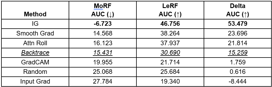
• LeRF AUC (Least Relevant First AUC): Evaluates how gradually perturbing the least important features (tokens) affects the model's confidence. The AUC measures the model’s response as the least relevant features are replaced with a baseline (e.g., [UNK]), indicating how much the model relies on these features.
• MoRF AUC (Most Relevant First AUC): Measures how quickly the model's performance deteriorates when the most important features are perturbed first. The AUC represents how the model's confidence decreases as the most relevant tokens are removed, revealing the impact of these key features on the prediction.
• Delta AUC: Represents the difference between LERF AUC and MORF AUC. It reflects how sensitive the model is to the removal of important features (MORF) versus less important ones (LERF). A larger delta suggests the explanation method effectively distinguishes between important and unimportant features.

The idea here is to attack the model on the most important tokens (as identified by DL Backtrace) and on the least important ones, and then compare how the prediction changes. From there, we build a graph of the model’s confidence in both scenarios, and the area between those curves gives us a measure of explanation quality.

Now, if you’re wondering how to try all this out—it’s actually quite simple.

With the free version of DL Backtrace, you can install the library, pass your model through it, and it will return the relevance values. From there, you can start interpreting your model and exploring how different parts of it contribute to its decisions. And if you want to quantify it, you can use our library as well - Xai_evals. 

pip install dl-backtrace
from dl_backtrace.tf_backtrace import Backtrace as B
backtrace = B(model=model)
layer_outputs = backtrace.predict(test_data[0])
relevance = backtrace.eval(layer_outputs, mode='default',scaler=1, thresholding=0.5, task="binary-classification")

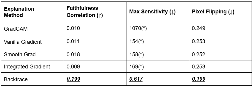
Benchmark: Image (ResNet-34)

Model description:

We used ResNet 34 Model which has :

• Basic blocks (two 3x3 convolutions per block).
• The exact block configuration of ResNet-34:
  
  • 3 blocks (64 filters), 4 blocks (128 filters), 6 blocks (256 filters), 3 blocks (512 filters).
• Downsampling at the start of stages 3, 4, and 5.‍
• Global average pooling and a fully connected layer for classification.

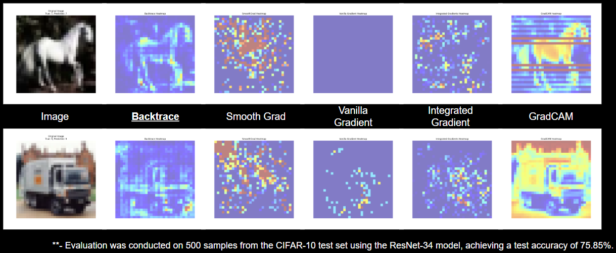
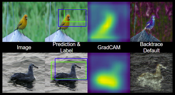
When you examine the visualizations, you'll notice that methods like Grad-CAM often assign high importance to nearly everything in the image. As a result, it becomes difficult to distinguish whether the model is actually focusing on the correct region for its decision or not. In some cases, the output may even appear blank or too diffuse to be interpreted meaningfully.

But with Backtrace, you can clearly see that it focuses on specific areas—particularly the edges and contours that actually drive the model’s decision. For example, if you look at the image of the horse, Backtrace doesn’t just highlight the body—it emphasizes the edges, the outline of the shape.

This tells us that the model is using the structural features of the object—like its silhouette—to make its prediction, rather than just relying on pixel intensity or broad regions.

Similarly, on the image side, we also evaluated Backtrace on segmentation and object detection tasks.

DLBacktrace on Segmentation Model

For segmentation, we treated these as ablation studies to gain a deeper understanding of the model’s behavior under different conditions.

We used the CleaningDB and Canvas datasets for this part of the evaluation.

ClinicdB Dataset:

We used custom U-Net Model involving a Conv Block (with two convolutional layers, BatchNorm, and ReLU activation) with Architecture:

1. Encoder: 4 downsampling levels (Conv2D + MaxPooling2D) with filters (32, 64, 128, 256).
2. Bridge: Bottleneck with 512 filters.
3. Decoder: 4 upsampling levels (Conv2DTranspose), skip connections, and conv_block.
4. Output: Single-channel Conv2D with sigmoid activation for binary segmentation.

CamVid Dataset:

We used a Classical U-Net:

1. Input: Shape (360, 480, 3).
2. Encoder: Downsampling with Conv2D layers (64, 128, 256 filters) and MaxPooling2D.
3. Bridge: Two Conv2D layers with 512 filters.
4. Decoder: Upsampling with Conv2DTranspose, skip connections, and Conv2D layers (256, 128, 64 filters).
5. Output: Single-channel Conv2D with sigmoid activation for binary segmentation.

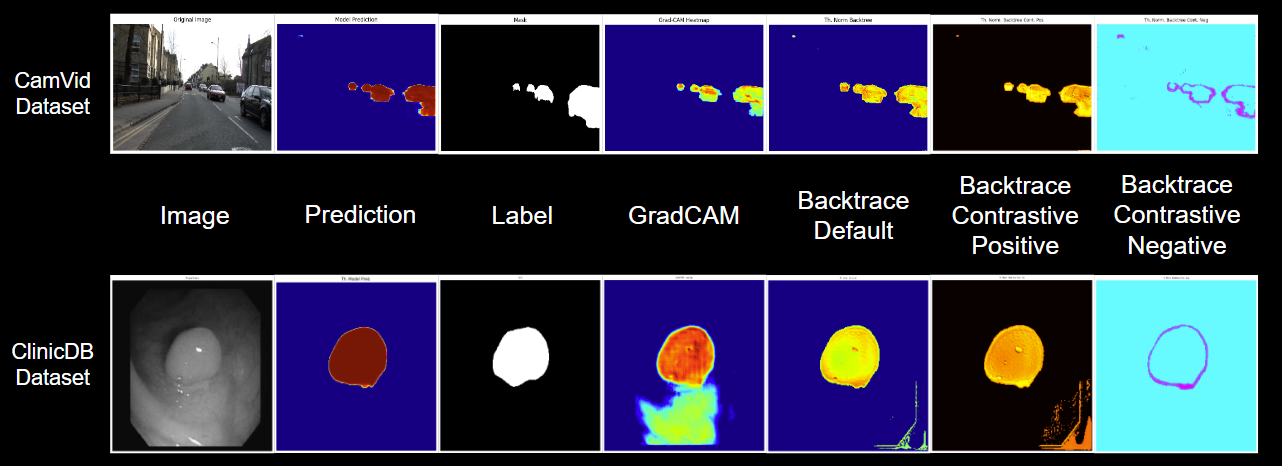
This is actually a great example of where contrastive mode shines. If you look at the Grad-CAM output, it tends to focus heavily on the interior of the object, assigning high relevance broadly—including to areas that aren’t critical for the decision. In some cases, the attribution appears excessive and not well localized.

In contrast, with Backtrace, the focus is much more precise—it highlights the edges and the exact regions that contribute to the model’s decision. When you view the positive relevance map, it clearly aligns with the areas driving the positive classification. And similarly, the negative relevance is also concentrated around the edges—indicating the regions that led the model to consider alternative or negative classifications. Importantly, it doesn't assign relevance to unrelated background areas.

This means you're getting focused, meaningful attribution—only for the parts of the image that actually matter.

DLBacktrace on Single Object Detection Model

Similarly, for the object detection task, we used a relatively lightweight model for evaluation. Model Architecture for Single Object Detection:

1. Input: Accepts an image of shape (224, 224, 3).
2. Convolutional Blocks:
   
   • 5 sequential blocks of Conv2D layers with ReLU activation and MaxPooling2D for feature extraction.
   • Filters progress as 32 → 64 → 128 → 256 → 512.
3. Global Pooling:
   
   • GlobalAveragePooling2D reduces spatial dimensions to a single vector.
4. Dense Layers:
   
   • Two fully connected layers with 512 and 256 units for feature refinement.
5. Output Layer:
   
   • Dense(4, activation='sigmoid') outputs 4 normalized values representing bounding box coordinates: [x_min, y_min, x_max, y_max].

If you look at the outputs from Grad-CAM and similar methods, you'll notice that the attributions are often blurry and lack fine-grained detail. It's difficult to pinpoint exactly what part of the image the model is relying on.

But with Backtrace, that’s not the case. You're able to see highly detailed and precise attributions, clearly highlighting the key features that influenced the detection.

This level of granularity can be extremely useful—not only for interpretability, but also for improving your model across a range of real-world applications.

Tabular Data

For the tabular task, we used a simple MLP model—essentially a basic neural network architecture.

Model Architecture:

• Input Layer: Identity layer, no transformation.
• Hidden Layers:
  
  • Three layers with sizes 78 → 39 → 19.
  • Each has ReLU activation and 20% dropout for regularization.
• Output Layer: Linear(19 → 1) with Sigmoid activation for probability output.

Despite its simplicity, the model's performance was quite strong, providing a solid foundation for evaluating the effectiveness of DL Backtrace.

And if you try this yourself using the free version of our library, you'll notice some clear differences—especially when comparing Backtrace with methods like LIME and SHAP. For example, with SHAP, it typically just selects the top 10 features, assigning high importance almost uniformly across them—regardless of context.

With LIME, it also selects top features, but does so based on the training distribution you provide. As a result, it often ends up assigning very high importance to those features, regardless of whether they’re relevant to the specific input. In SHAP's case, the issue is that it tends to assign some importance to almost all features, which can dilute the explanation.

So in both cases, these methods lack instance-specific precision. If everything is marked as important, then essentially nothing is, and the explanation loses value.

Backtrace, on the other hand, avoids this problem by providing more focused and accurate attributions, tailored to the actual instance being evaluated. Try it out for yourself—you’ll see the difference.

With that, let’s move on to the BERT model.

Experiment BERT Model Description

We used the textattack/ bert-base-uncased-SST-2 model, a fine-tuned version of BERT (Bidirectional Encoder Representations from Transformers) tailored for binary sentiment classification on the Stanford Sentiment Treebank (SST-2) dataset.

Model Architecture:

- Base Model: BERT-base-uncased, comprising 12 Transformer layers, each with 768 hidden units and 12 attention heads, totaling approximately 110 million parameters.

- Fine-Tuning: The model includes an additional classification layer on top of the `[CLS]` token's output, producing logits for binary sentiment classes (positive or negative).

‍Tokenizer:

- Utilizes the BERT-base-uncased tokenizer, which processes text into lowercase and applies WordPiece tokenization, ensuring compatibility with the model's pre-training.

For the BERT experiments, we used a pre-trained TextAttack model on the Stanford Sentiment Treebank (SST-2) dataset, which is a standard benchmark for binary sentiment classification—positive or negative.

Input:

The emotions are raw and will strike a nerve with anyone who's ever had family trauma

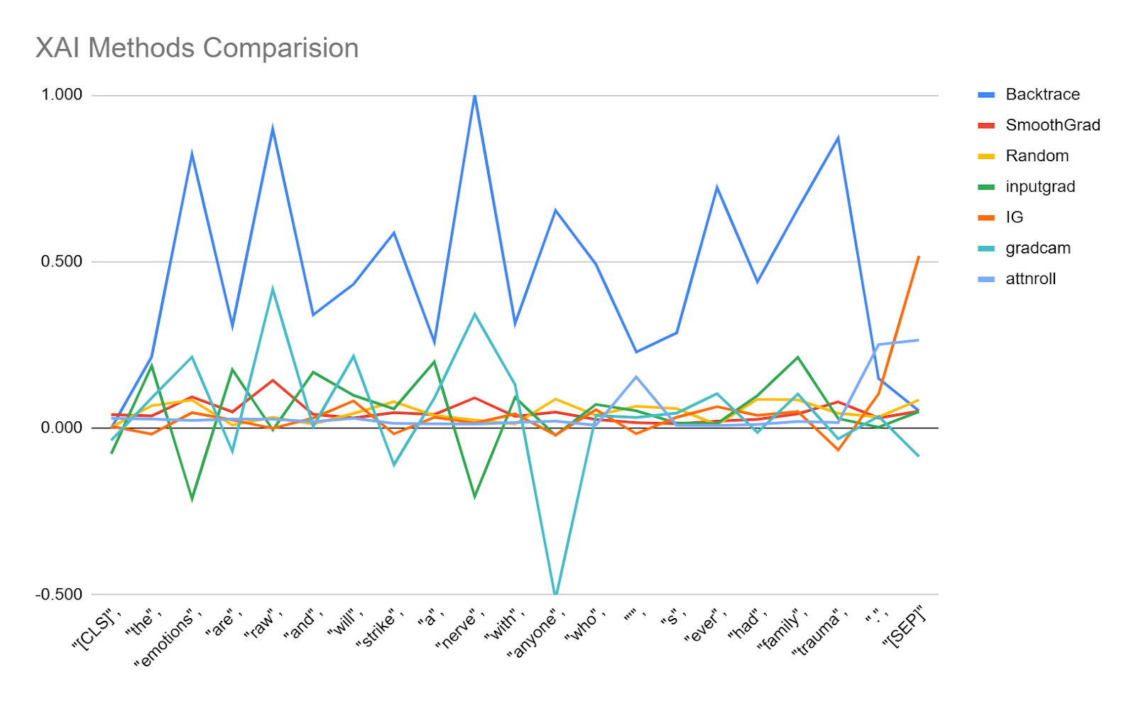
Output:

• Prediction : 1
• Label : 1

So, what can we conclude from all this?

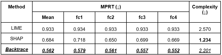
• For tabular models, Backtrace demonstrates superior MPRT scores compared to LIME and SHAP.
• While it may have slightly higher computational complexity, that’s a tradeoff for more granular and accurate explanations.
• For image-based tasks, Backtrace outperformed all other methods across key metrics.
  This makes it especially suitable for high-stakes applications, where fine-grained attributions are critical.
• For text, IG is currently better in terms of benchmark metrics, but Backtrace is rapidly improving, with promising results already emerging.

In fact, we’ve also tested Backtrace across a range of text tasks and models:

• On T5, LLAMA, and Con1D (a compact modular classification model), the results were insightful.
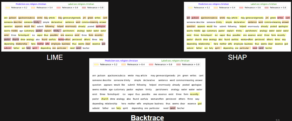
  For example, in the Con1D case, Backtrace focused on a very small subset of meaningful words, whereas LIME and SHAP distributed relevance across almost every word, making interpretation less actionable.

DLBacktrace on Embedding + Conv1D Model

Text classification model with:

1. Input: Takes string input.
2. Processing: Converts text to vectors using vectorizer and embedding_layer.
3. Convolutions: Three Conv1D layers with 128 filters and MaxPooling1D for feature extraction.
4. Pooling: GlobalAveragePooling reduces dimensions.
5. Dense Layers: Fully connected layer with 128 units, 50% dropout, and a softmax output for len(class_names) classes.

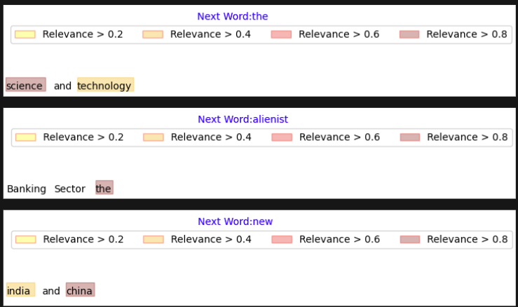
DLBacktrace on LSTM Model

LSTM-based model for Next Word Text Generation has:

1. Embedding Layer: Maps tokens to 64-dimensional vectors.

2. LSTM Layer: Captures sequential dependencies with 100 units.

3. Dropout Layer: Prevents overfitting with 10% dropout.

4. Dense Output: Predicts the next word using `softmax` over `total_words` (vocabulary size).

In a next-word prediction task using an LSTM-based model, say for a news headline like "science and technology", Backtrace accurately highlighted the core content words, rather than spreading importance evenly.

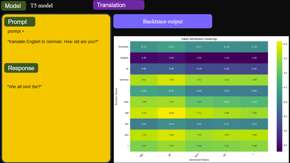
• For T5 translation, Backtrace allowed us to trace which input tokens contributed most to the generation of each output token—a valuable tool for sequence-to-sequence analysis.

• And with LLAMA, we tested a sentiment analysis task where the model classifies text into positive, negative, or neutral.

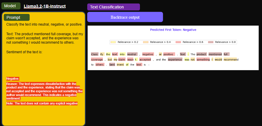
Here too, Backtrace effectively focused on the task-relevant tokens—like "classify," "positive," and "neutral"—while ignoring irrelevant stop words, producing a sharp and focused explanation.

Overall, these results show that Backtrace is not only generalizable across modalities and tasks, but also provides meaningful, instance-level attributions that are easy to interpret and useful in practice.

Notebook Walkthrough

The session also included a notebook walkthrough demonstrating how DL Backtrace works with models like LLaMA 3.2, OLMV, and JetMOE (a Mixture-of-Experts model).

Using JetMOE as an example, the walkthrough showed how DL Backtrace can trace token-level relevance—such as identifying specific terms like "function," "nth," and "Fibonacci" as key contributors to a generated response. The tool also provides layer-wise relevance graphs, helping users visualize which self-attention and feedforward layers play a more significant role in model predictions.

In Mixture-of-Experts models, DL Backtrace can pinpoint which expert paths were most influential, allowing users to prune less-relevant experts for domain-specific tasks, leading to lighter and more efficient models.

The same relevance-tracing capabilities were demonstrated on OLMV and LLaMA, particularly for sentiment classification tasks, showing how token and layer importance can guide model optimization and transparency.

Overall, the walkthrough highlighted how DL Backtrace helps in understanding which layers, tokens, or experts are critical for a decision—enabling more explainable, aligned, and efficient model deployments.

Why DL Backtrace?

So, why choose Backtrace over methods like LRP, GradCAM, or Integrated Gradients (IG)?

As you've seen, Backtrace enables full-network analysis. It doesn't just highlight a few features—it helps you understand underlying patterns, such as biases in your dataset, or where uncertainty might influence predictions.

It provides feature importance at both the local level—specific to individual predictions—and the global level, by aggregating explanations across multiple samples. This dual perspective gives you a comprehensive understanding of your model’s behavior.

Another key advantage is efficiency. Unlike perturbation-based methods, Backtrace is deterministic. There's no need for repeated inferences or sampling. You get the entire explanation in a single pass, making it much faster and more stable for large-scale use.

‍Limitations of DLBacktrace:

• Computational Cost: Scales linearly with model depth. Batch processing is recommended for large datasets.
• Model Access Required: Needs full access to model weights and architecture. Not applicable to true "black-box" models without workarounds.

Despite these, for use cases where model access is possible, Backtrace offers a robust, scalable, and interpretable solution for understanding deep learning systems.

Recap:

• DLBacktrace is a novel and robust method that significantly improves deep learning model interpretability.
• It provides clear, consistent, and reliable insights into feature importance and information flow.
• Outperforms existing methods in robustness and accuracy across various model types.
• Promotes responsible AI deployment in critical applications by enhancing model transparency and trustworthiness.

Q&A section:

Sugun Sahdev:
Thank you so much, Pratinav, for that insightful presentation. We’re now opening the floor for questions.
Our first question is:
“What is our advantage compared to the competition?”

Pratinav Seth:
Great question. The key advantage of DL Backtrace is that it provides reliable, deterministic explanations, unlike methods like LIME or SHAP that rely on surrogate modeling. With Backtrace, you can confidently explain how the model arrived at its prediction—even to a regulator—because it's not a black box.
It doesn't change behavior on similar inputs, and it allows you to justify decisions with a clear trace of which features contributed most.

Sugun Sahdev:
Next: “What strategic advantages does DL Backtrace offer over traditional interpretability methods like SHAP or LIME, especially in high-stakes domains like finance or healthcare?”

Pratinav Seth:
Both finance and healthcare require trustworthy and explainable models. The issue with SHAP and LIME is that they use surrogate models, based on input-output behavior, which opens them up to scaffolding attacks—making them less credible to regulators.
Backtrace, on the other hand, is deterministic and architecture-aware. It operates directly on model weights, so it can’t be easily tricked and gives a more robust and trustworthy explanation.

Sugun Sahdev:
Another question: “Can DL Backtrace work affordably on large models like ChatGPT, and how long does it take?”

Pratinav Seth:
Currently, Backtrace doesn't support closed-source models like ChatGPT, since it requires access to model weights.

However, for open-source models like LLaMA, it's fully functional. At the moment, you can get explanations in 1–2 minutes per instance, and we’re actively optimizing for real-time performance.
Eventually, we aim to have it run in parallel with inference, minimizing additional overhead.

Sugun Sahdev:
“Are relevance scores computed independently for each layer, or is there a layer-wise dependency?”

Pratinav Seth:
Relevance is computed for each layer and operation, including neuron-wise detail. While there's some layer-wise dependency, we’ve built it to support almost all standard layers in PyTorch—about 95% of real-world models are covered.
Only highly custom or CUDA-optimized layers might pose issues.

Sugun Sahdev:
Here’s one more: “How does Backtrace compare to SAEs in terms of scalability?”

Pratinav Seth:
SAEs are useful but extremely resource-intensive—you have to train them for each model.
With Backtrace, there’s no training involved. It works directly on the pretrained model and computes relevance during inference. So, in terms of scalability, Backtrace is significantly more efficient and practical for large deployments.

Sugun Sahdev:
“Can DL Backtrace help assess hallucinations or token-level failures in generative models?”

Pratinav Seth:
Yes, we’re actively researching that. With Backtrace, you get layer-wise relevance values, which can help identify spikes or anomalies during hallucinations.
We’ve seen a pattern in our results linking high relevance in specific layers to potential failures or hallucinations. This can also inform pruning and alignment strategies. More results on this are coming soon.

Sugun Sahdev:
“Is Backtrace similar to LRP?”

Pratinav Seth:
In principle, yes—they both aim to compute relevance.
But LRP uses different rules for different layers, making it harder to scale.
Backtrace uses a single rule across all layers, making it simpler, consistent, and scalable. We support both default and contrastive modes, without requiring complex configurations.

Sugun Sahdev:
“How do I choose between default and contrastive modes?”

Pratinav Seth:
Default mode works well for most general use cases.
Use contrastive mode when you want to understand why a decision was made by looking at positive vs. negative contributions.
It's especially helpful in classification boundaries or nuanced decision points. We showed default mode in our demo, but contrastive often gives deeper insights in sensitive use cases.

Sugun Sahdev:
“Can Backtrace be used for factuality correlation to neurons, like Anthropic’s SAE work on LLMs?”

Pratinav Seth:
Yes, though the approach differs.
Anthropic uses sparse autoencoders, which are slow and complex to train.
Backtrace instead computes neuron-level relevance directly. So yes, you can use it for factuality correlation, but through a relevance-based approach instead of SAE-style training.

Sugun Sahdev:
“Are there any architectural limitations—e.g., does it require monotonic or smooth activations?”

Pratinav Seth:
Not really. You can use any standard activation function—even custom ones—as long as they’re properly defined.
Only very rare cases, like custom CUDA kernels, may be tricky to integrate. But for 95% of PyTorch-based models, Backtrace works out of the box.

Sugun Sahdev:
“Can you quantify these explanations across methods, like MPRT for LLMs?”

Pratinav Seth:
Yes! We’ve built a library called XAI Evals that supports metrics like MPRT and others.
While it’s currently more focused on MLPs, it can be extended to LLMs too.
There’s a lot of scope for new evaluation methods, and we’re happy to see community contributions as well.

Sugun Sahdev:
Last one: “Are there opportunities for students to be involved in research or projects?”

Pratinav Seth:
Absolutely! We’ve had several student interns over the last six months working on explainability, alignment, and practical applications of Backtrace.

We’re very open to collaboration and usually aim for at least one publication per student.
Feel free to reach out—we’re always excited to support new researchers.

Sugun Sahdev:
That brings us to the end of today’s webinar.
Thank you all once again for joining us—we hope this session helped you better understand DL Backtrace and its potential to bring trust and transparency into deep learning systems.

Take care, and we look forward to seeing you in future sessions!